01
Which customers are likely to adopt?
Estimate household-level ownership probability from income, education, commuting, housing and other characteristics.
GIM estimates which representative households are most likely to own EVs, develops charging requirements from travel and charging assumptions, and adds those loads to existing whole-home 8,760 profiles.
The same number of EVs can produce different grid consequences depending on where owners live, how far they travel, when they return, charger power, charging frequency and coincidence with existing household demand.
Estimate household-level ownership probability from income, education, commuting, housing and other characteristics.
Translate travel distance and vehicle assumptions into required charging energy rather than assuming every EV charges identically.
Use arrival timing and selected behavior assumptions to place charging within the customer’s hourly load profile.
Add EV kW to air conditioning, heating, water heating, appliances and other coincident residential demand.
Each step preserves customer and time differences before results are aggregated to utility planning geographies.
Select the service-area ownership scenario for the current year, 2030 or 2035.
Calculate an EV probability for each representative customer using nearest-neighbor analysis.
Convert travel, arrival and charger assumptions into customer hourly charging loads.
Combine EV charging with each customer’s existing whole-building 8,760 profile.
Produce customer, neighborhood, block-group, ZIP and service-area results.
A household can have a high probability of EV ownership but create different hourly impacts depending on driving, arrival time, charging power and existing load. GIM models those relationships in sequence instead of treating adoption and peak kW as one average assumption.
The utility-wide EV scenario controls the overall ownership level. Customer probabilities determine where ownership is allocated, and charging profiles determine when the new demand appears.
The non-parametric nature of a K-nearest-neighbor (KNN) model can identify local ownership and commuting patterns missed by the more rigid parametric structure of traditional statistical models.
The method works directly from observed similarities among households.
Model estimation requires a reliable training" database including households with and without EVs.
A Level 2 charger may draw 11.5 or more kilowatts, but the relevant planning quantity is the diversified, coincident charging load added to existing customer demand.
Longer daily travel generally increases required charging energy and potential charging duration.
Arrival patterns determine whether charging begins before, during or after the residential and G&T peak.
Higher charger capacity increases instantaneous load but may shorten the charging period.
EV charging must be evaluated alongside AC, heat, water heating, appliances and other customer demand.
Not every EV starts charging at the same time, requires the same energy or remains at full charger output for the same duration.
Time-of-use and managed charging can delay, stagger or shift demand, but can also create rebound or synchronized start effects.
The original Rhode Island example demonstrates why averages must be interpreted carefully. Individual customers show different charging start times and durations, lowering the average ZIP-level kW contribution relative to one charger’s maximum draw.
However, filtering the same area for higher-propensity customer characteristics revealed a neighborhood segment with substantially greater EV ownership and whole-home load impacts than the ZIP average.
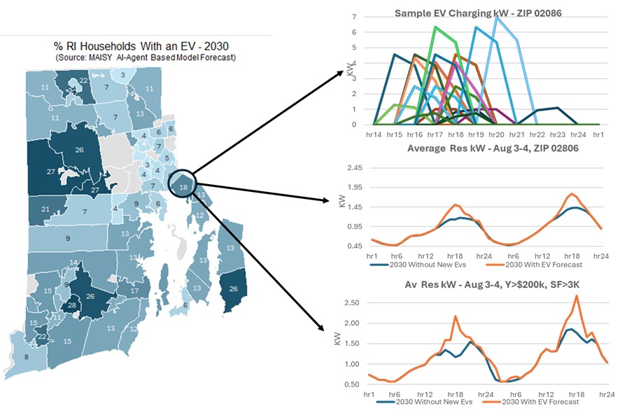 Open the original EV charging kW graphic full size ↗
Confusing charger nameplate kW with diversified or coincident EV load can materially distort both grid-risk and business-case results.
The maximum charging rate available from the equipment under applicable vehicle and circuit limits.
The load of an EV that is actively charging at a particular hour; it may be below nameplate.
Charging load averaged across all EV owners, including vehicles not charging during the hour.
The EV contribution during the utility, feeder, neighborhood or transformer peak being evaluated.
EV charging plus the customer’s baseline residential demand at the same hour.
The charging contribution remaining after participation, availability and control effectiveness are applied.
The ownership and charging models supply a common analytical foundation for the expanded GIM worksheets.
Compare customer, block-group, ZIP and service-area ownership and load impacts.
Apply localized EV peak loads with utility-selected size, current loading and planning-limit assumptions.
Supply priority-area 8,760 profiles to CYME, Synergi, WindMil, OpenDSS and other workflows.
Compare unmanaged, time-of-use and controlled charging with participation and engagement assumptions.
Translate coincident kW reduction into avoided G&T demand charges, payback, benefit-cost ratio and NPV.
Evaluate EV charging alongside weather-sensitive loads, batteries and other flexible resources.
Because not every EV charges simultaneously or at maximum power. Required energy, arrival time, charger limits and charging duration create diversity that must be modeled.
It estimates EV ownership probability for each identity-protected representative household by comparing that household with similar records in the EV ownership calibration database.
GIM applies commuting distance and selected vehicle and charging assumptions to estimate the energy that must be restored and the hours over which charging occurs.
Transformers and feeders experience total customer demand, not EV charging alone. Air conditioning, heating and other household loads determine the actual coincident impact.
Yes. GIM scenarios allow key EV growth, charging and program assumptions to be revised so utilities can compare alternatives rather than rely on one forecast.
No. It provides planning-level screening, prioritization and hourly inputs. Asset-specific thermal, voltage, protection and reliability analysis remains an engineering function.
Request a guided demonstration of customer probabilities, charging profiles, whole-home loads and current GIM applications.